
HySP: Hyper Spectral Phasor
This software is designed and scripted using Python 3.5 and PyQt5. The nature of the software inspires its multi-platform portability. We currently have Windows and MacOSX versions.
Latest Version:
| OS | Download | Size |
|---|---|---|
| MacOSX (tested 10.11+) | HySP-0.9.20.dmg | 406.7MB |
| Windows 64bit (tested Windows 7 64bit) | HySP-0.9.18-amd64.msi | 368.7MB |
Thanks for downloading our Software! Before you do, we would like to know who you are, where you are and what sort of data you will be analyzing. After you fill out the following form, it will take you to the download page.
You should know that by downloading the software, you are agreeing to use it for research only and you cannot use for a commercial purpose.
If you use our software to analyze the data and publish a paper, that's great and we would like you to acknowledge the software in the paper. We would also like you to send us a citation reference to the paper so we know we are doing good.
Installation Instructions:
Windows: download .msi installer, double click and follow wizard instructions.
Mac: download .dmg image, drag app to Application folder.
Typical Install time: 2 minutes.
Sample Datasets (general):
Here are 2 sample datasets for testing the software. Datasets were acquired using Zeiss LSM 710 and LSM 780 with Meta/Quasar mode.
- Zebrabow_x_hspCre_26hpf_brains_458-561-1frame-1024.lsm
- Wildtype_autofluorescence-20hpf-750nm-brightfield.lsm
Main datasets used in SEER publication (SEER: Nature Communications Vol 11, Article num: 726 (2020) doi: 10.1038/s41467-020-14486-8):
- fig1_140117 oct nang E12_2015_03_14__19_34_20__t006.lsm (2.08 GB) [ubi:Zebrabow multispectral, Zeiss 780 Quasar, 40x 1.1NA W, Excitation: 458nm laser, Detection: 32 wavelength bins, 8.9nm bandwidth, 410-695 nm range]
- fig2-3_newCheckerboard_20180516.tif (6.0 MB) [Simulated Hyperspectral Test Chart (SHTC) built from real microscopy data of CFP, YFP, RFP transgenic zebrafish, Zeiss 780 Quasar, 40x 1.1NA W, Excitation: 458nm laser, Detection: 32 wavelength bins, 8.9nm bandwidth, 410-695 nm range]
- fig4_HySP_1frameHD_740nm_pos2.lsm (67 MB) [freshly isolated mouse tracheal explant, multispectral, Zeiss 780 Quasar, 40x 1.1NA W, Excitation: 740nm laser, Detection: 32 wavelength bins, 8.9nm bandwidth, 410-695 nm range]
- fig5_02-mko2-wholefish-FL.lsm (3.0 GB) [Zebrafish - Tg(fli1:mKO2) pan-endothelial fluorescent protein label, multispectral, Zeiss 780 Quasar, 40x 1.1NA W, Excitation: 488nm laser, Detection: 32 wavelength bins, 8.9nm bandwidth, 410-695 nm range]
- fig6_27-fish3-ct122a-kdrl-mcherry-cerulean-458nm-tile-zoom-forcomparison.lsm (3.0 GB) [Zebrafish Tg(kdrl:eGFP); Gt(desmin-Citrine);Tg(ubiq:H2B-Cerulean), multispectral, Zeiss 780 Quasar, 40x 1.1NA W, Excitation: 458nm laser, Detection: 32 wavelength bins, 8.9nm bandwidth, 410-695 nm range]
- fig7_fish1_tileHD_Brain_zoomout2x.lsm (133 MB) [Zebrafish ubi:Zebrabow, multispectral, Zeiss 780 Quasar, 40x 1.1NA W, Excitation: 458nm laser, Detection: 32 wavelength bins, 8.9nm bandwidth, 410-695 nm range]
- Simulations (10.2 MB) [Simulation of 3 fluorescent spectra at different overlap level and different signal to noise, Detection: 32 wavelength bins, 8.9nm bandwidth, 410-695 nm range]
Main datasets used in Hybrid Unmixing publication (HyU: currently under review):
- Figure 2 Folder
(A,B) Multispectral simulations of four fluorophore patterns - includes no optical filter and optical filter, Detection: 32 wavelength bins, 8.9nm bandwidth, 410-695 nm range (115 MB) (E) Zebrafish 10 dpf muscle - Gt(cltca-Citrine); Tg(ubiq:lyn-tdTomato; ubiq:Lifeact-mRuby; fli1:mKO2), Zeiss 780 Quasar, 40x 1.1NA W, Excitation: 458nm and 561 nm laser, Detection: 32 wavelength bins, 8.9nm bandwidth, 410-695 nm range (1.09 GB)
- fig3_02-fish10-zoom-FL-zstack.lsm (1.00 GB) [Zebrafish 2 dpf trunk region- Gt(cltca-Citrine); Tg(ubiq:lyn-tdTomato; ubiq:Lifeact-mRuby; fli1:mKO2), multispectral, Zeiss 780 Quasar, 40x 1.1NA W, Excitation: 458nm and 561 nm laser, Detection: 32 wavelength bins, 8.9nm bandwidth, 410-695 nm range]
- Figure 4 Folder [Zebrafish 5 dpf mid-body to tail region - Gt(cltca-Citrine); Tg(kdrl:mCherry; fli1:mKO2) timelapse files, multispectral, Zeiss 780 Quasar, 40x 1.1NA W, Excitation: 740nm laser, Detection: 32 wavelength bins, 8.9nm bandwidth, 410-695 nm range]
- Figure 5 Folder
(A) Zebrafish 3 dpf whole sample - Gt(cltca-Citrine); Tg(ubiq:lyn-tdTomato; ubiq:Lifeact-mRuby), multispectral, Zeiss 780 Quasar, 40x 1.1NA W, Excitation: 488nm and 561nm laser, Detection: 32 wavelength bins, 8.9nm bandwidth, 410-695 nm range (1.95 GB) (B) Zebrafish 3 dpf head region - Gt(cltca-Citrine); Tg(ubiq:lyn-tdTomato; ubiq:Lifeact-mRuby) + strong autofl, multispectral, Zeiss 780 Quasar, 40x 1.1NA W, Excitation: 488nm and 561nm laser, Detection: 32 wavelength bins, 8.9nm bandwidth, 410-695 nm range (8.70 GB) (E) Zebrafish 3 dpf head region - Gt(cltca-Citrine); Tg(ubiq:lyn-tdTomato; ubiq:Lifeact-mRuby) + strong autofl, multispectral, Zeiss 780 Quasar, 40x 1.1NA W, Excitation: 740nm laser, Detection: 32 wavelength bins, 8.9nm bandwidth, 410-695 nm range (8.43 GB)
- fig6_02-fishtail-timelapse-6points-fl488561.lsm (32.0 GB) [Zebrafish 3 dpf tail region - Gt(cltca-Citrine); Tg(ubiq:lyn-tdTomato; ubiq:Lifeact-mRuby) + strong autofl, multispectral, Zeiss 780 Quasar, 40x 1.1NA W, Excitation: 458nm and 561 laser, Detection: 32 wavelength bins, 8.9nm bandwidth, 410-695 nm range]
Convert Wavelength to RGB (Python)
This function is adapted from Dan Bruton's work
Reference HySP:
If you use HySP for your work or publication, please cite it as:
Hyperspectral phasor analysis enables multiplexed 5D in vivo imaging
Francesco Cutrale, Vikas Trivedi, Le A Trinh, Chi-Li Chiu, John M Choi, Marcela S Artiga & Scott E Fraser
Nature Methods 14, 149–152 (2017) doi:10.1038/nmeth.4134
Link
Reference SEER:
If you use SEER for your work or publication, please cite it as:
Pre-processing visualization of hyperspectral fluorescent data with Spectrally Encoded Enhanced Representations
Wen Shi, Daniel E. S. Koo, Masahiro Kitano, Hsiao J. Chiang, Le A. Trinh, Gianluca Turcatel, Benjamin Steventon, Cosimo Arnesano, David Warburton, Scott E. Fraser & Francesco Cutrale
Nature Communications volume 11, Article number: 726 (2020) doi: 10.1038/s41467-020-14486-8
Link Open Access
License
HySP and SEER follow the University of Southern California and Translational Imaging Center Software License available here .
Instructions
These instructions were written by Wen Shi and Francesco Cutrale at University of Southern California on 2019-03-30
Introduction
HySP is a multi-platform software for analysing multi-dimensional data. The application here uses hyper- and multi-spectral datasets. The software calculates a 2D phasor plot which can be analyzed interactively with ROI selectors, both phasor-to-image and image-to-phasor. The denoising algorithm improves the quality of data by reducing poissonian noise.
SEER is a pre-processing visualization approach for hyper- and multi-spectral fluorescent images. The technique is incorporated in the HySP software platform, a multi-platform software for analysis of multi-dimensional spectral data. SEER provide rapid enhanced visualization of spectral datasets, starting from fluorescent data.
Starter Guide / README
This is a Starter Guide including updates on SEER (Spectrally Encoded Enhanced Representations) [Starter Guide SEER]
This is a Starter Guide including updates on Hybrid Unmixing (HyU) [Starter Guide HyU]
Detailed Guide PDF
This is a Detailed Guide of HySP including updates on SEER and HyU in pdf format [Detailed Guide PDF]
Command window
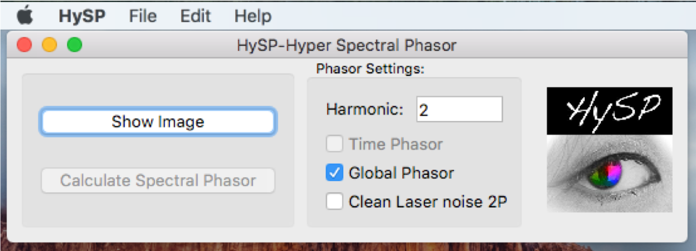
After opening HySP software, the command window shows as below.
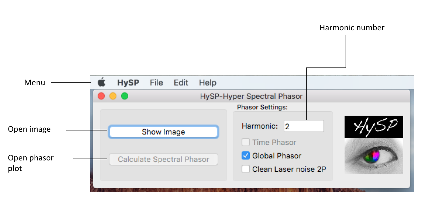
Menu
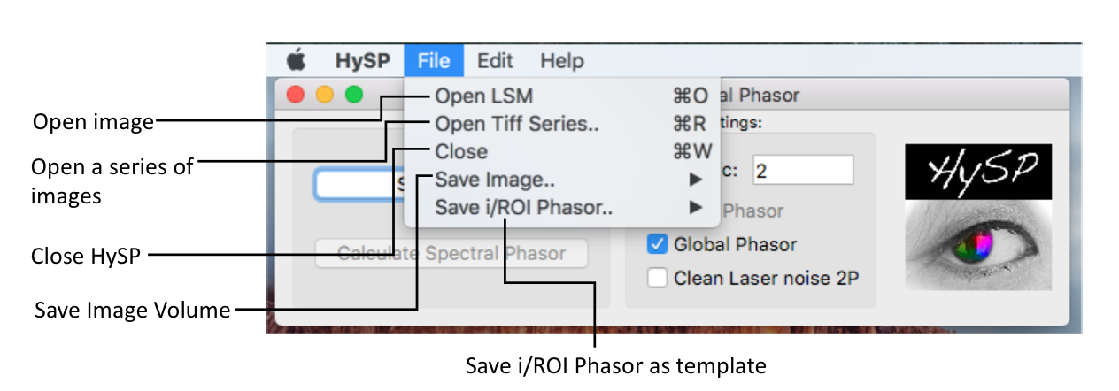
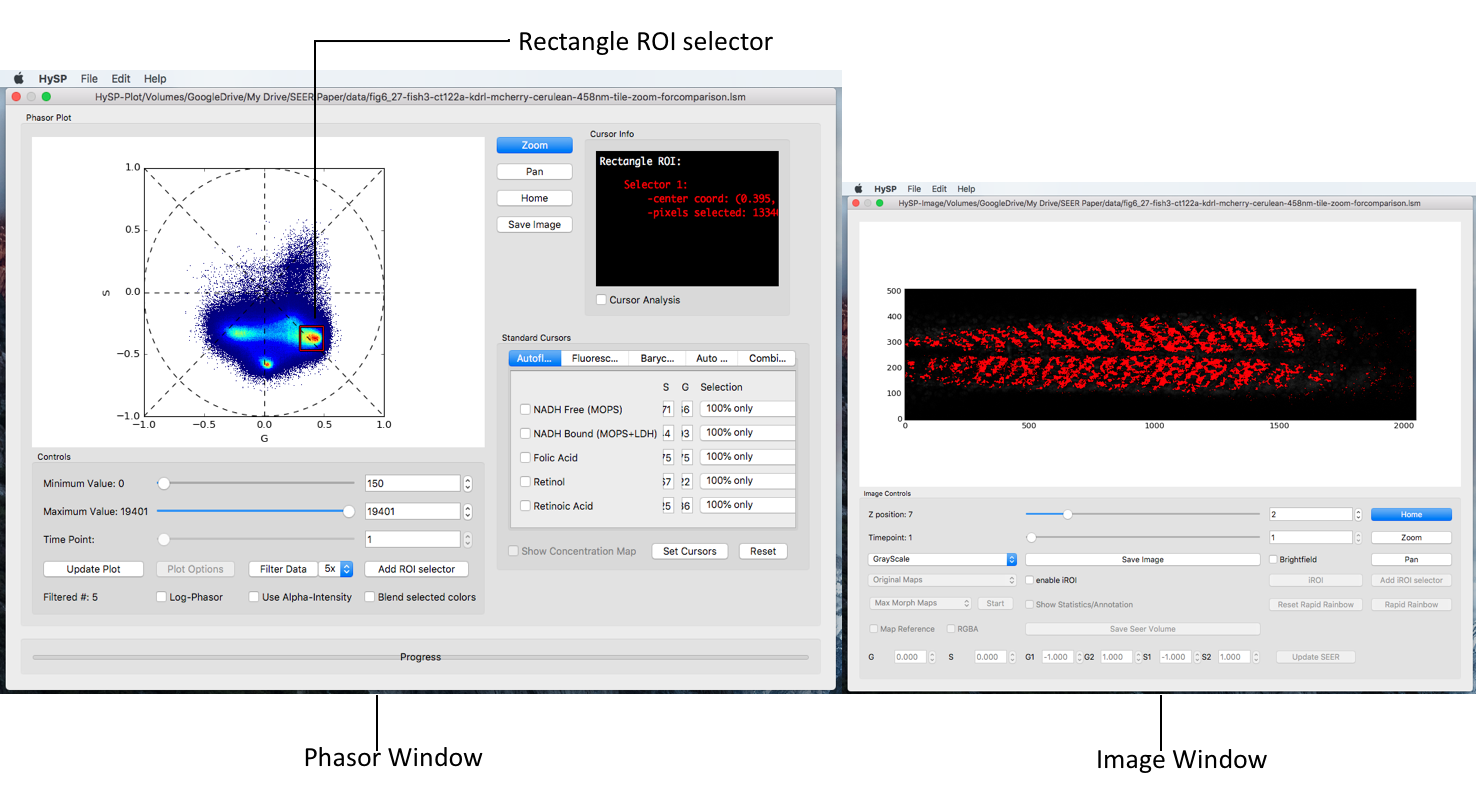
Image window
Phasor window
Set up HySP software
Harmonic
In the command window, under Phasor Settings the harmonic number can be typed. (i.e. harmonic:1; default configuration is 2)
Loading images
As of now HySP supports .lsm and .tiff files. Tiff files should be in a single tiff sequence or multiple multi-layer tiff files. NOT all layers in a single tiff file. Example: if dataset has shape [time, z-stack, channel, x, y] then it should be saved as one multi-layer tiff for each channel or each z-stack [t, :, ch, :,:] , or [t, z, :, :,:]
1. Open .lsm file
Click Show Image > choose the file (file in .lsm format) > click Open .
File > Open LSM >choose the file (file in .lsm format) > click Open .
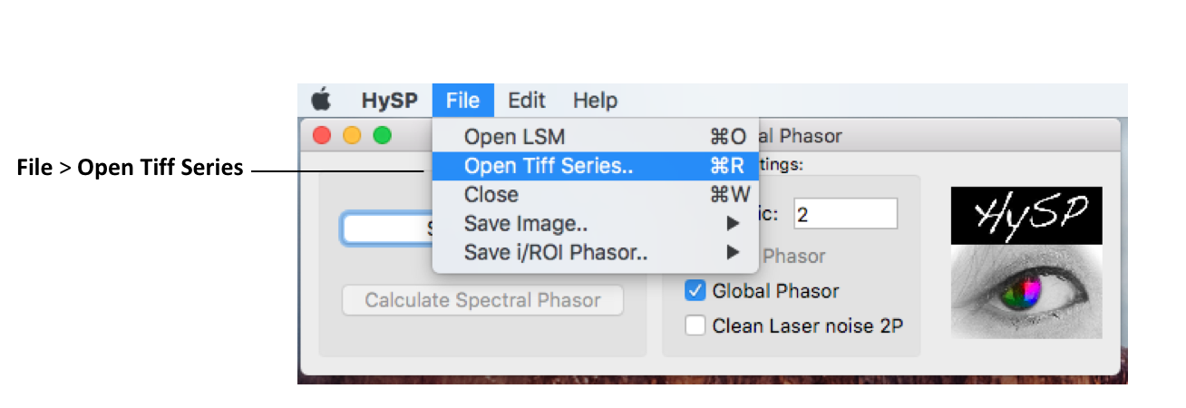
2. Open generic .tiff file
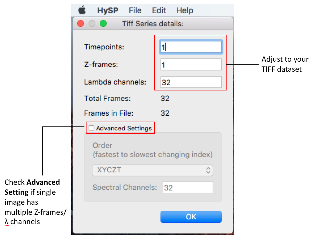
File > Open Tiff Series > set up Tiff Series Details window.
Detailed info on dataset shape can be set in the window as below, parameters can be edited according to user's data.
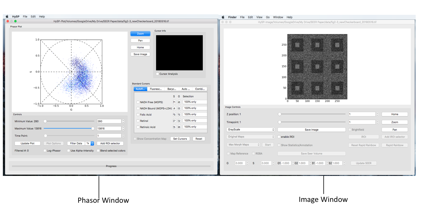
Open Spectral Phasor window
On to the commend window > Click Calculate Spectral Phasor.
The phasor window shows as below.
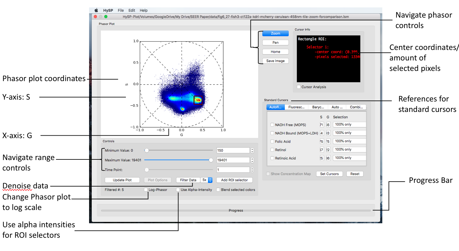
Working with Phasor
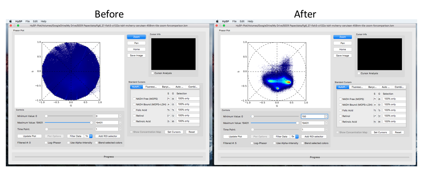
Filter
Click Filter Data/SDenoise to reduce noise in phasor plot. This step can be repeated up to 10 times to improve phasor quality.
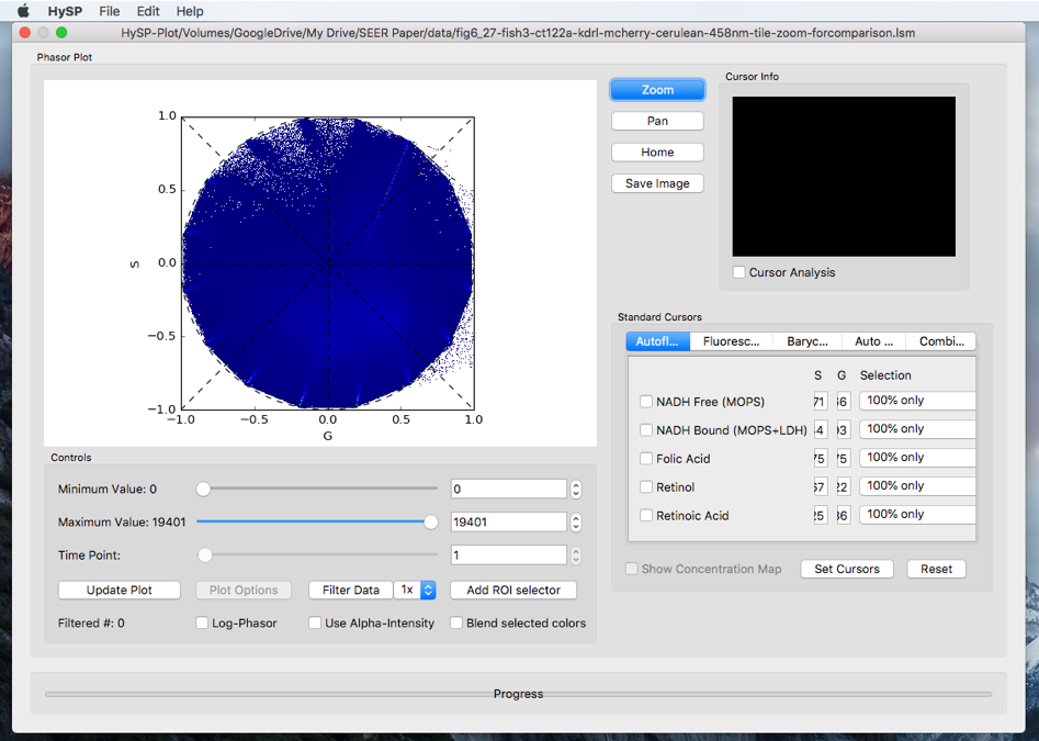
Range controls
Type in Minimum Value, Maximum Value > Click Update Plot to view fluorescent pixels in interested range.
Here is a comparison of filtering and range controlling
Scale controls
Select Log-Phasor checkbox to visualize the phasor in log-scale. Click Update Plot to update window.
ROI controls
Select Use Alpha-Intensity checkbox to represent ROI phasor selection as an alpha-overlay on top of the image in Image Window. This visualization mode creates a colormap black-to-[color of ROI] and maintains the intensity of the underlying pixel. Generally useful for visual representation/rendering. Use Alpha-Intensity applies to all the ROIs added after the checkbox selection. Default mode (uncheckedg Use Alpha-Intensity) is a solid color represenation.
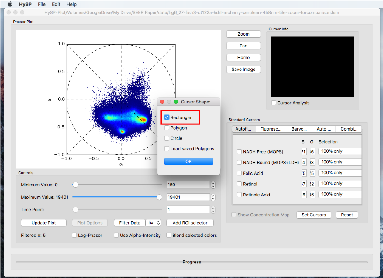
ROI selector
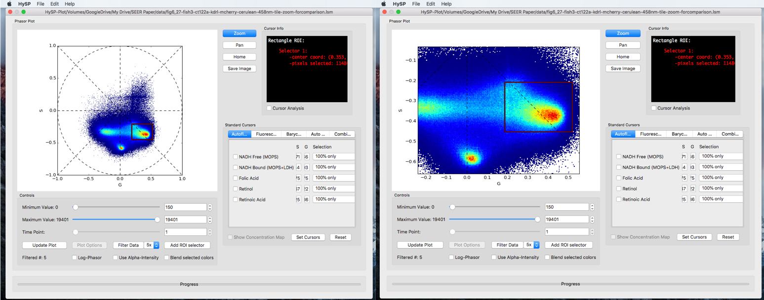
Rectangle
Rectangle ROI selector can acquire the coordinates in Cursor Info window;
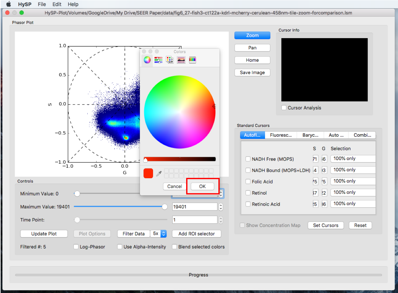
Click Add ROI selector > Choose the options, i.e. Rectangle > Click OK > Choose the color > Click OK > Move the rectangle on phasor.
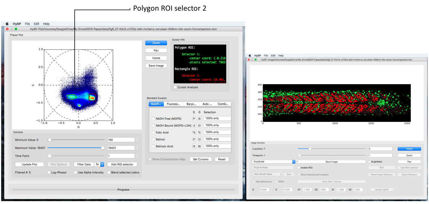
Note: The phasor window and the image window can be viewed the same time to see the phasor chosen by rectangle is in which part of specimen in image. The specimen in image will be marked the same color user has chosen for rectangle in previous step.
Step1. Add ROI Selector
Step2. Selector color
Step3.
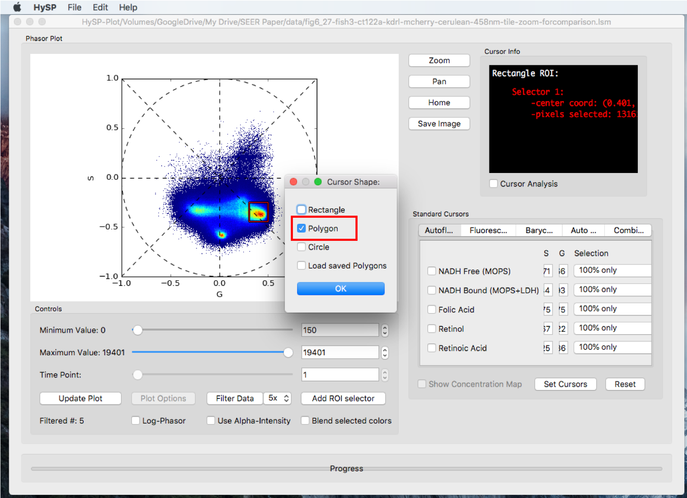
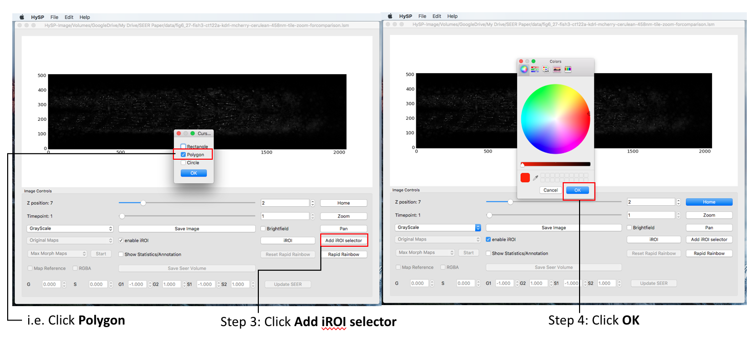
Polygon
Click Add ROI selector > Choose the options, i.e. Polygon > Click OK > Choose color > Click OK > Right click to move the polygon; Left click inside polygon close to vertices to change the shape.
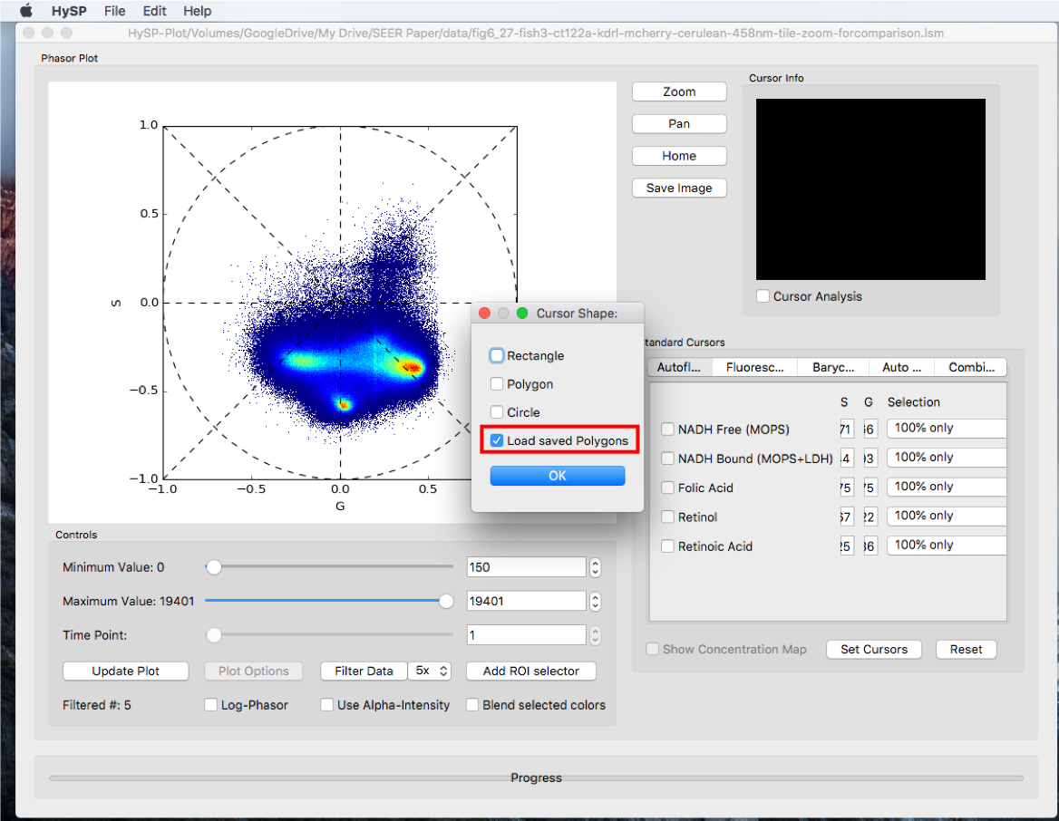
Load Saved Polygons
Click Load Saved Polygons and load previous polygons as template.
Navigating Phasor plot
Zoom
Click Zoom, frame the region surrounding the area of interest and zoom into it.
Click Zoom again to lock the region in case the phasor plot moves.
Home
Click Home to get the original zoom factor.
Pan
Click Pan to traslate S and G direction on the phasors.
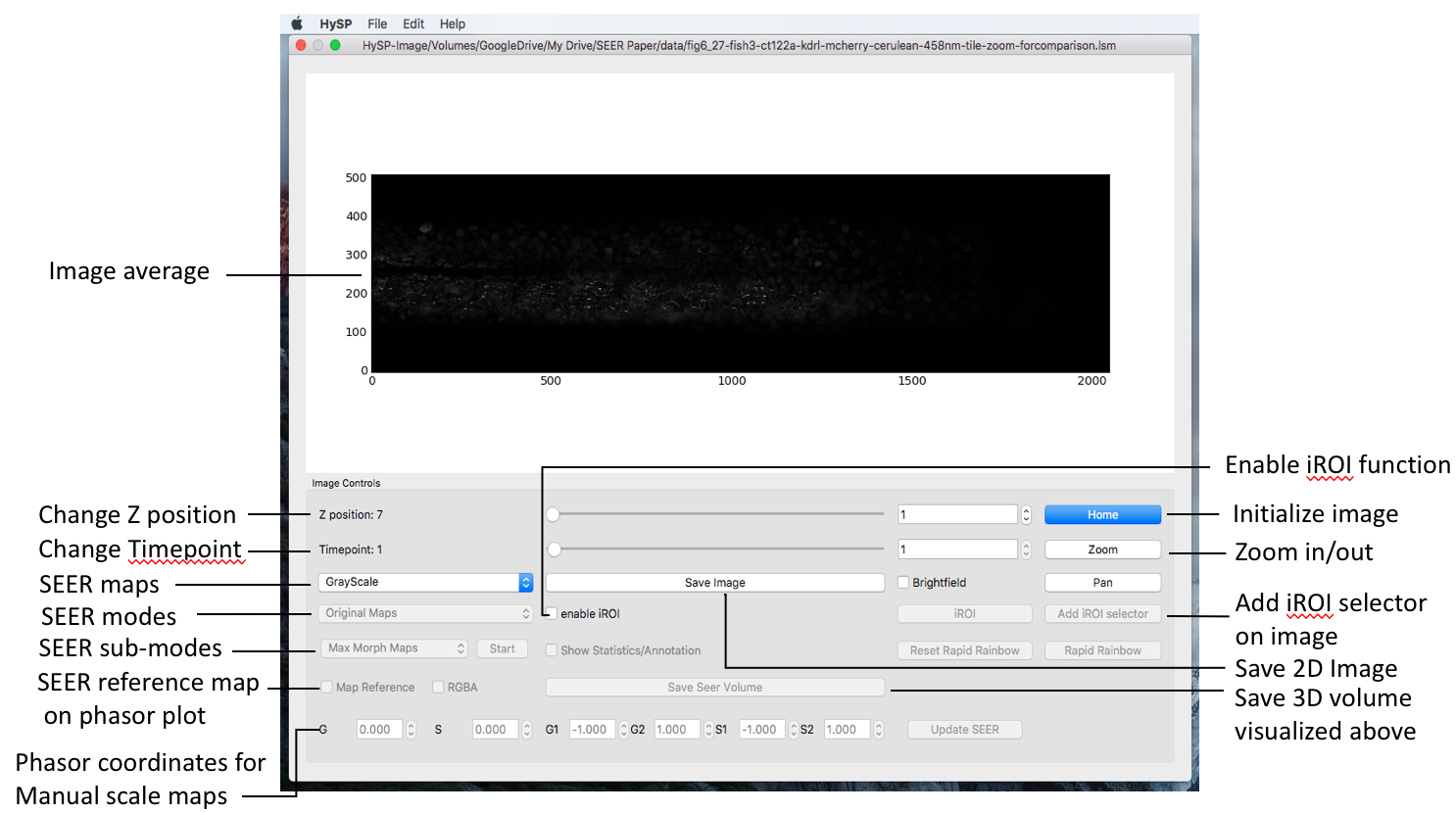
3D datasets [z,lambda,x,y] and 4D [t,z,lambda,x,y]
Scroll Z-position in Image Window to visualize the chosen volume slice in dataset.
Scroll Timepoint in Image Window to change time position in dataset.
Cursor info
For rectangle ROI and iROI, center coordinates are reported in >Cursor Window.
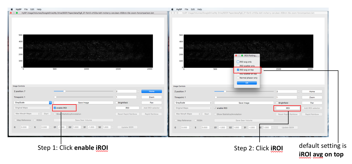
iROI selector
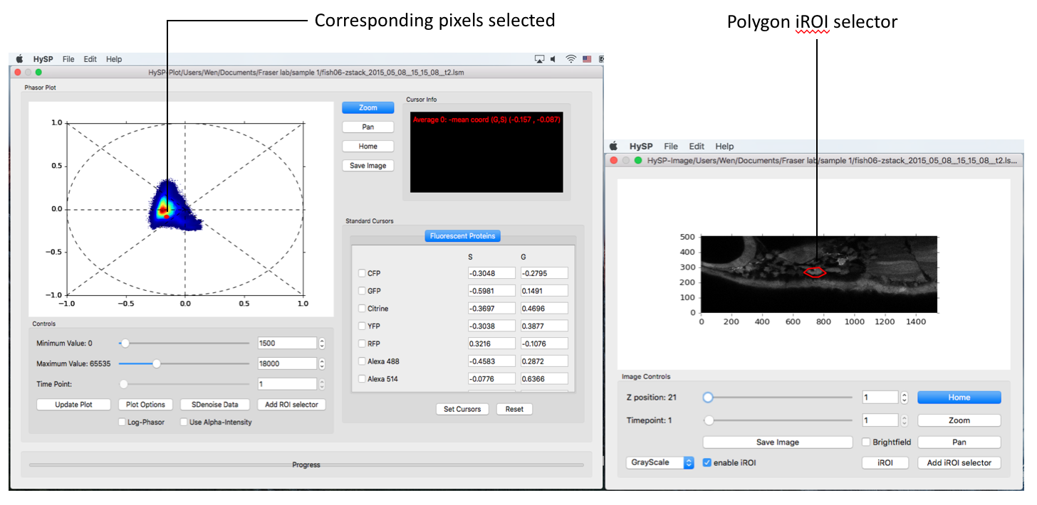
This option enables an ROI selector on the Image (rather than on the phasor). The (S,G) values of each pixel selected on the image are then reported on the phasor according to the modality selected. E.g. average (S,G) with std for G and S axis.
In Image Window Choose enable iROI > Click iROI options and choose (i.e. iROI avg on top) > Click on iROI >Choose cursor options (i.e. Polygon) > Select color (red as default) > Click OK > Move polygon on interested area > Statistics are reported on Cursor Info tab and in Phasor plot in Phasor window.
Note: Multiple polygons can be added on image with different colors, the area selected is labelled the same color in Phasor plot.
The iROI selector is represented with the same color on top of the phasor plot
Note: To load a new image and acquire the phasor of that image, you need to close all the windows and reopen HySP
Saving Data, ROIs and Images
Save Data
Processed data can be saved as .TIFF multilayer files by pressing File > Save Volume.. > Save Image Volume..
Each channel will be saved as a separate file. Each file will contain an entire z-stack if present. Multiple timepoint will contain t__ in filename
Save ROIs
ROIs selections on phasor can be saved by pressing File > Save i/ROI Phasoe.. > Save ROI Phasor as..
The file saved can be then reloaded on a different dataset by clicking on Add ROI in Phasor Window and selecting Load ROI.
Save Images
Each image can be saved as a color picture (*.png). On Phasor Window > Save Image.. will save the phasor canvas with ROIs as currently visualized.
On Image Window > Save Image.. will save the image currently represented in the image canvas.
SEER Visualization
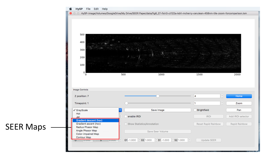
SEER Maps
After loading data and applying denoising, return to the Image window and on the bottom left click on the dropdown menu labeled “Grayscale” and the different SEER options of Gradient ascent, descent, radius, angle, and contour will appear.
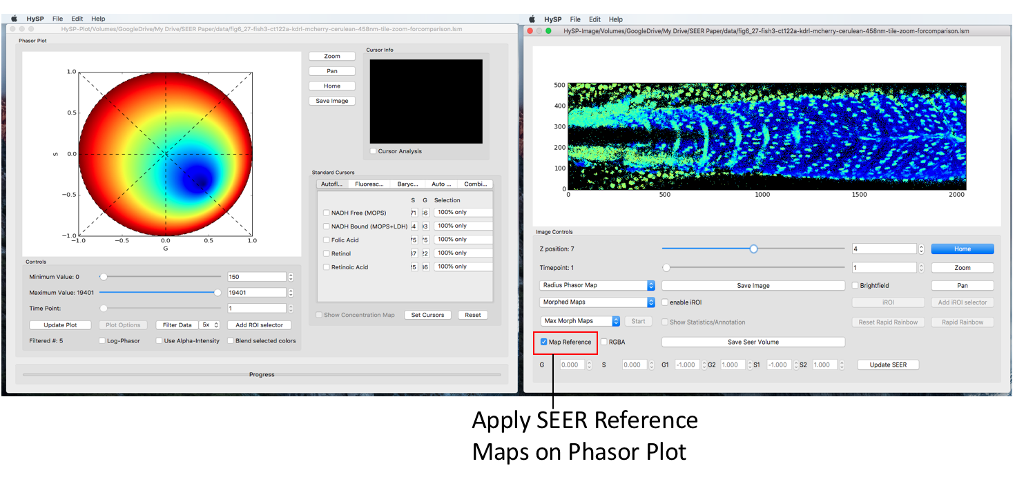
SEER Reference Maps
Toggle the Map Reference checkbox, corresponding reference map will be updated on phasor window.
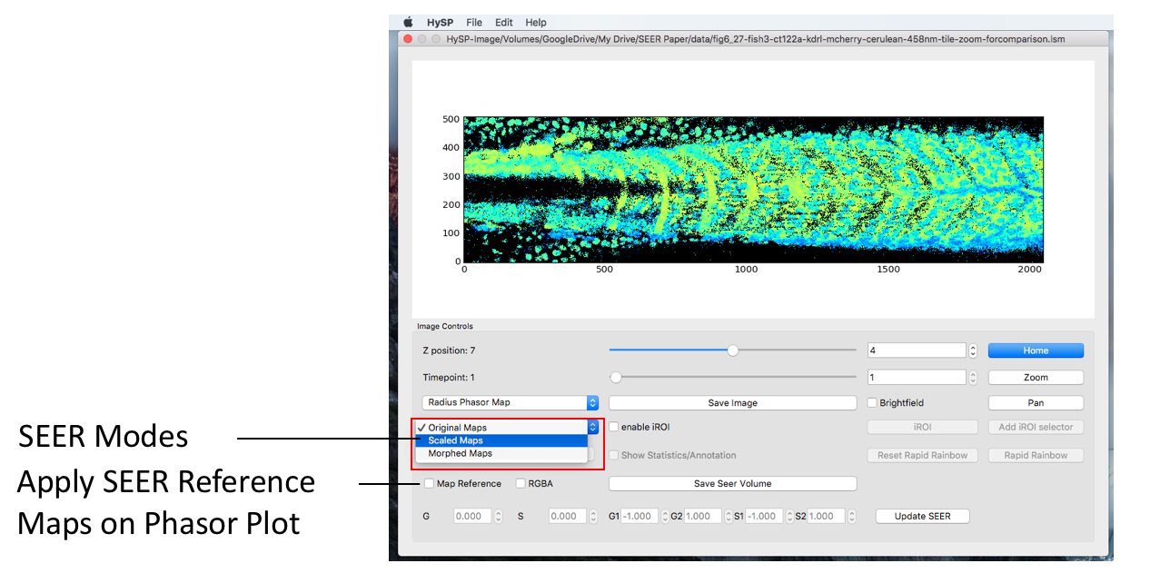
SEER Modes
The “Mode” dropdown menu is right below the SEER map menu. The initial value is set as “Original Maps” and there are “Scaled Mode” and “Morphed Mode” available.
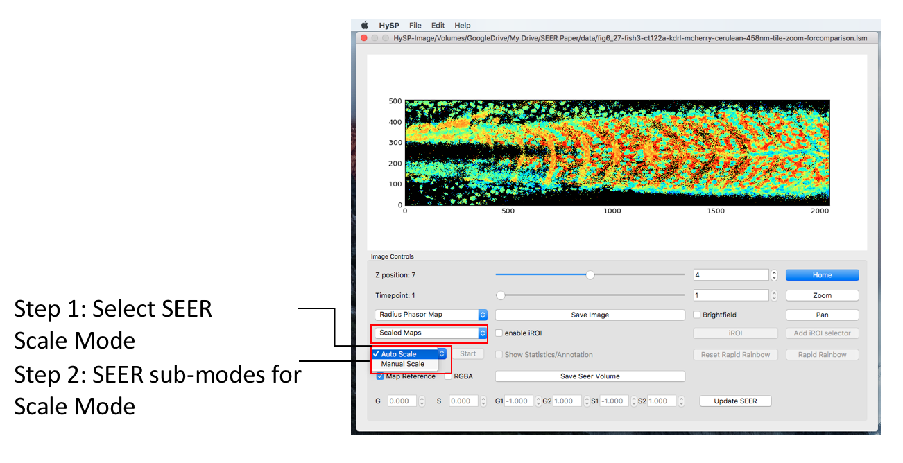
Scale Mode
Under Scaled mode there are auto-scale and manual scale mode.
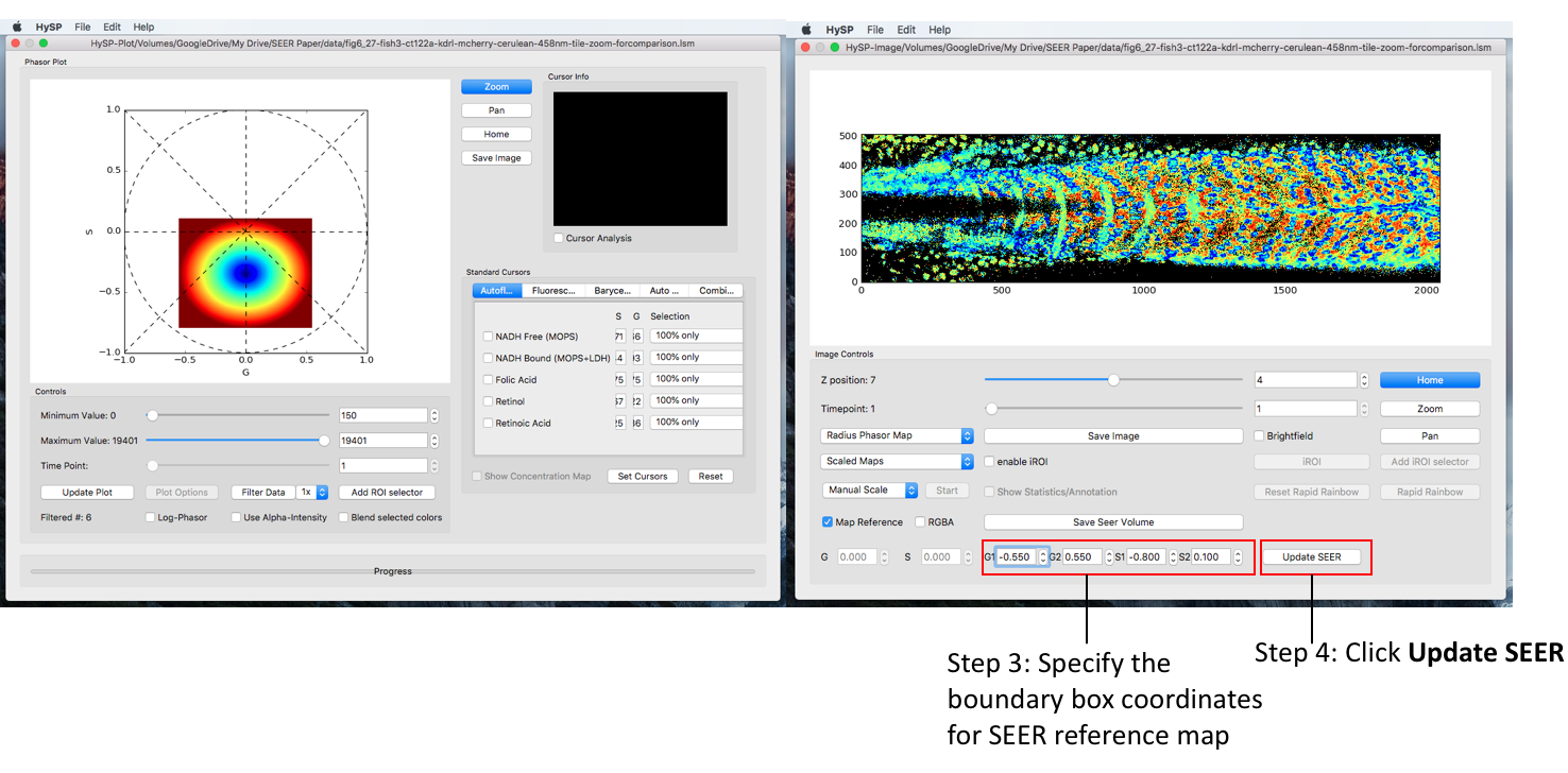
Manual Scaled Mode
Selecting “Scaled Maps” will enable the sub-modes for this mode.
One can type in the G/S values to specify the reference map position on phasor plot, click Update SEER to scale and relocate the map reference on phasor plot. See figure below.
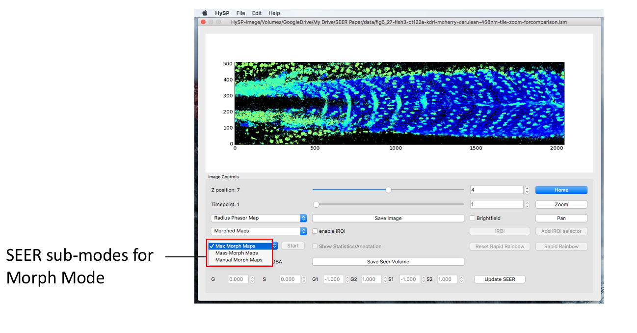
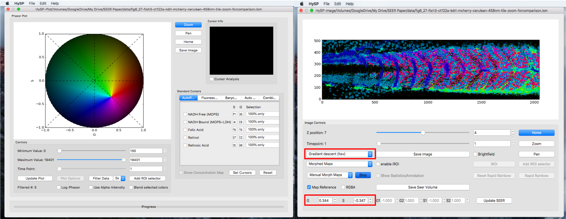
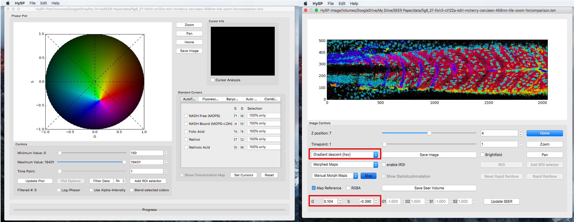
Morph Mode
Under Morph mode, there are Max Morph mode, Mass Morph mode, and Manual morph mode. As an example, selecting Morphed Maps in the “Mode” dropdown menu will activate the different Morph modes in the drop down right below.
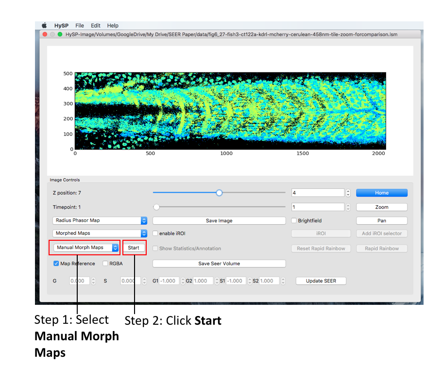
Manual Scaled Mode
Select Morphed Maps,Manual Morph Maps to activate manual morph mode. Click Start.
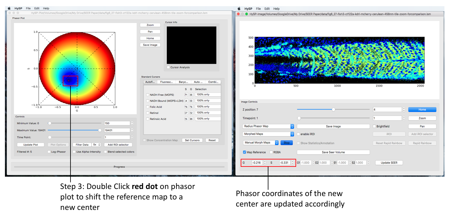
Mouse double click on phasor plot to morph the map reference to a new center, (G, S) coordinate of this new center is also updated when mouse released.
To explore the dataset, one can always switch to another map under any mode and sub-mode.
Save Volume Image
Click Save Seer Volume will yield a series of Tiff files in a name required folder for future processing, i.e. 3D rendering.
eN&B tools
This calibration tool is designed for calculating parameters necessary for accurate analysis Calibration_Utility-20200420.zip .
Here is an example file for dark
This tool is designed for calculating eNB
eNB-Windows7.zip
eNB-Windows10.zip .
Here is an example file for data
eN&B Reference
If you use this tool for your work or publication, please cite it as:
Eph-ephrin oligomerization and signaling modulated by receptor polymerization-condensation
Ojosnegros S., Cutrale F., Rodriguez D., Otterstrom J.J., Chiu C., Hortigela V., Tarantino C., Seriola A., Mieruszynski S., Martinez E., Lakadamyali M., Raya A., Fraser S.E. . PNAS, 114 (50) 13188-13193 (Dec. 2017) DOI